Training a Multi-Camera Flow Matching Policy for Robot Pouring

I have been spending time learning robot learning from the ground up: starting in simulation before moving to a physical robot arm on my desk.

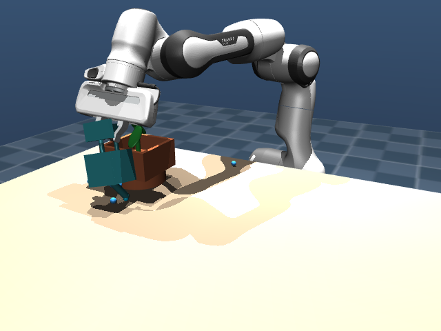
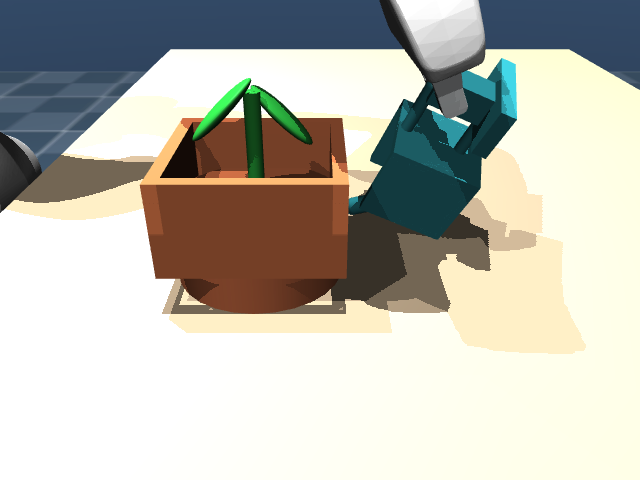
To understand how modern continuous-control policies actually behave beyond basic pick-and-place tutorials, I built FloraFlow: a PyTorch and MuJoCo codebase where a 7-DoF Franka arm grasps a watering can by its narrow 8 mm handle, carries it across a desk, and tilts it to pour water into a plant pot.

My first pixel-to-action policy worked 75% of the time when the objects spawned near their training positions, but failed 70% of the time (dropping to 30% success) as soon as I shifted the watering can and plant pot 5 to 10 cm outside the training bounds. This note documents what it took across 14 ablation runs to reach 100% success on those out-of-distribution shifts, and what showed up when I built a visualizer to peer inside the network.

The Setup

The simulation runs MuJoCo physics at 500 Hz while the policy runs at 20 Hz (one decision every 50 ms). At each step, the model sees:

• Three synchronized $128 \times 128$ RGB cameras: third_person_cam, overhead_cam, and a wrist-mounted wrist_cam.
• Nine proprioceptive values: 7 joint angles, gripper finger width, and episode phase progress.

Instead of predicting a single motor step at a time, the policy predicts a chunk of the next 16 steps ($0.8\text{ s}$ ahead) using Optimal Transport Conditional Flow Matching (OT-CFM). ¹ 1. Unlike diffusion policies that denoise along curved stochastic paths, Optimal Transport Flow Matching regresses a straight velocity vector field $\mathbf{x}_1 - \mathbf{x}_0$ between Gaussian noise and the target action chunk. At inference time, 10 simple Euler steps take about 5.2 ms on my Mac.

@torch.no_grad()
def sample_action_chunk(model, obs_embedding, num_steps: int = 10):
    x = torch.randn((obs_embedding.shape[0], 16, 8), device=obs_embedding.device)
    dt = 1.0 / num_steps
    for step in range(num_steps):
        t = torch.full((obs_embedding.shape[0], 1), step * dt, device=x.device)
        v = model.predict_velocity(x, t, obs_embedding)
        x = x + v * dt
    return x

What Worked and What Failed

Instead of guessing at hyperparameters, I logged 14 training runs testing data volume, image shift augmentation, multi-camera cross-attention, and bottleneck size.

Run	Change Tested	In-Distribution (20 Seeds)	Hard OOD (50 Seeds)	Spout Error (ID / OOD)
Run 5	Baseline (100 demos, no augmentation)	75% (15/20)	30% (6/20)	16.3 cm / 31.5 cm
Run 6	Add $\pm 4\text{ px}$ random image shifts	85% (17/20)	34% (17/50)	10.5 cm / 23.5 cm
Run 7	Scale to 300 demos + dual cameras	90% (18/20)	80% (40/50)	10.0 cm / 12.0 cm
Run 9	Add 3rd camera + Cross-Attention (320-dim bottleneck)	100% (20/20)	72% (36/50)	7.7 cm / 15.1 cm
Run 12	Compress bottleneck (16 keypoints/cam, 192-dim)	95% (19/20)	100% (50/50 Clean)	8.7 cm / 8.5 cm
Run 14	300 collision-cleaned demos + lr=5e-4	100% (20/20)	90% (45/50 Clean)	8.1 cm / 13.3 cm

Why a Smaller Visual Bottleneck Beat a Larger One

The most interesting surprise happened between Run 9 and Run 12.

In Run 9, I added the third camera and fused the views with 4-head cross-attention into a 320-dimensional bottleneck (using 32 SpatialSoftmax keypoints per camera). ² 2. Spatial Softmax turns each convolutional feature map into an expected 2D pixel coordinate $(u, v)$, giving the policy explicit 2D spatial points instead of a flattened feature vector. In-distribution performance hit 100%, but Hard out-of-distribution performance actually dropped from 80% down to 72%.

When I inspected the failed rollouts, the reason was clear: with 32 keypoints per camera and a wide 320-dimensional bottleneck, the MLP had enough capacity to memorize static background coordinates on the table. When the watering can moved outside the training region, those memorized correlations broke.

In Run 12, I cut the keypoints in half (from 32 down to 16 per camera) and squeezed the fused bottleneck from 320 down to 192 dimensions. Forcing the visual state through a tighter bottleneck stopped the network from memorizing background pixels and forced it to track relative geometry between the gripper, the handle, and the pot. Hard OOD success jumped to 100% (50/50 on collision-free spawns).

Seeing Inside the Policy

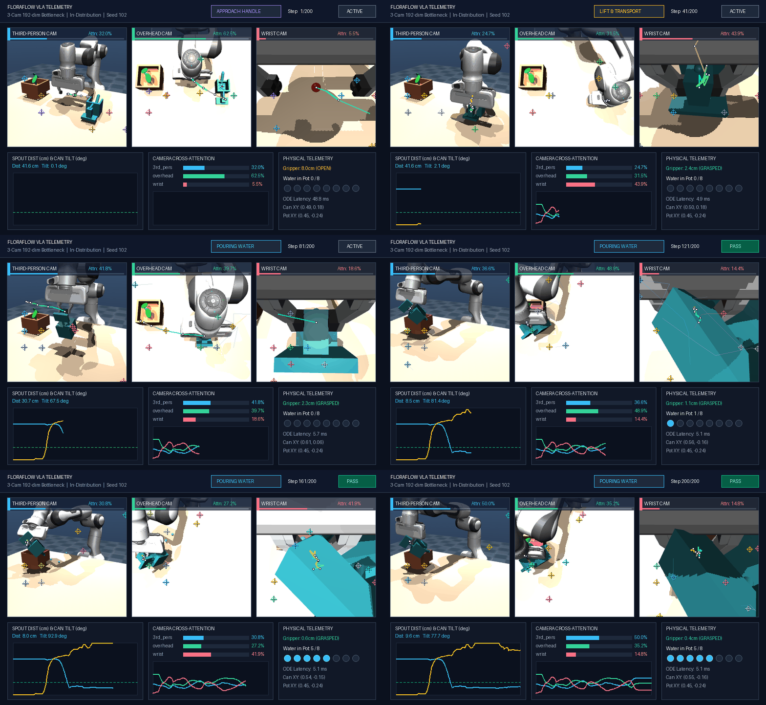
Debugging a vision policy by only watching whether the robot succeeds or fails is frustratingly opaque. I wrote a diagnostic HUD (VisionRolloutVisualizer) that renders four things at every frame:

1. 2D Spatial Keypoints (+): The highest-confidence SpatialSoftmax points, which lock onto the plant leaves, can handle, and wrist.
2. Predicted 3D Trajectory Ribbon: The 16 future joint steps passed through forward kinematics and projected into each camera’s 2D view.
3. Camera Cross-Attention Weights: A live bar chart showing which camera the policy trusts at each moment.
4. Physical Task Metrics: Spout-to-pot distance and tilt angle.

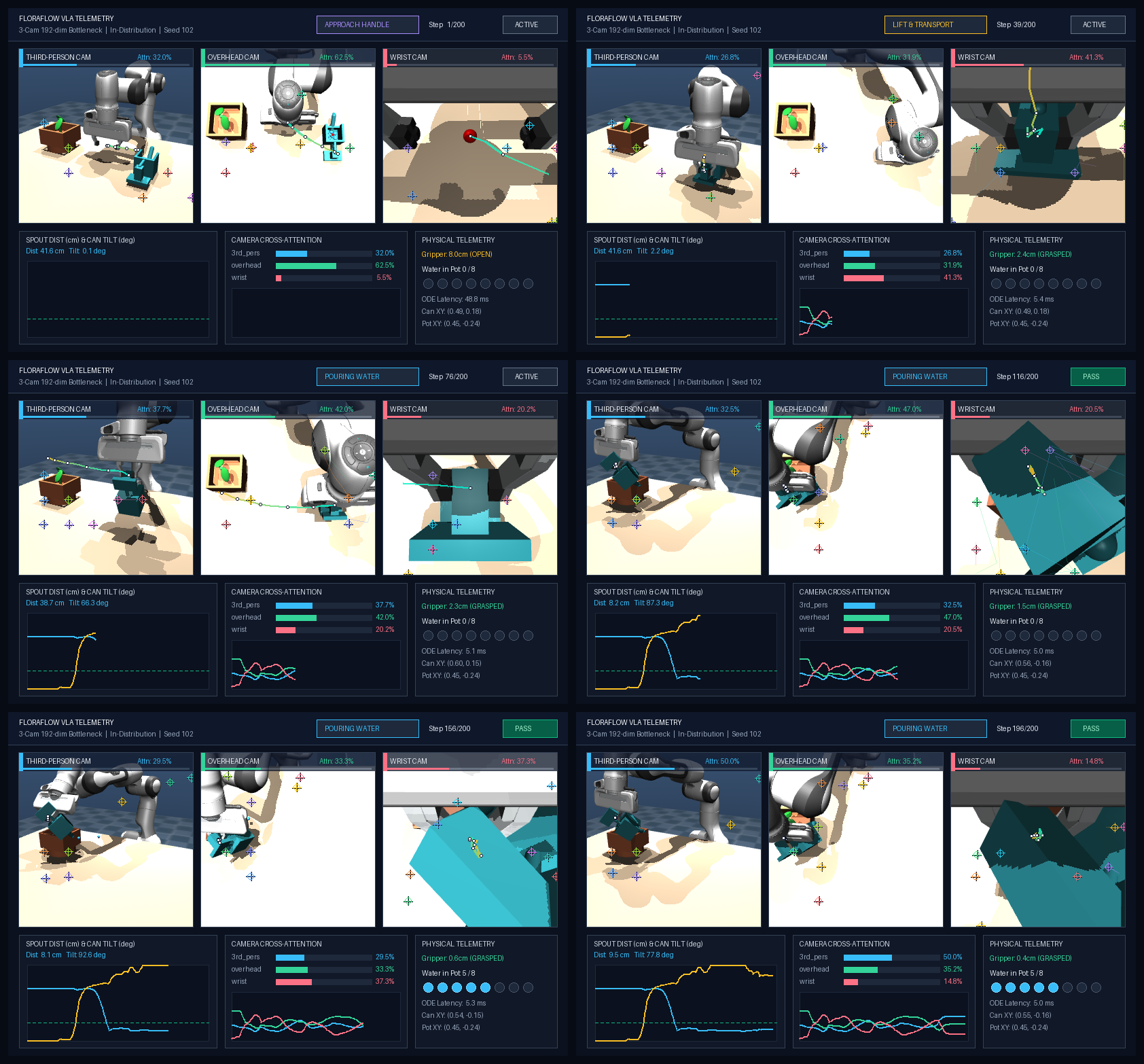
Watching the cross-attention bars during a rollout revealed behavior I never explicitly programmed:

• Approach (Step 1): The policy puts 62.5% of its attention on overhead_cam to line up global $(X, Y)$ coordinates over the table.
• Handle Grasp (Step 39): As the fingers close around the 8 mm handle, wrist_cam attention spikes to 51.8% for fine alignment.
• Pouring (Steps 116 to 196): When the arm tilts the watering can to 85 degrees, the can’s body blocks the wrist camera’s view. The policy automatically shifts 85% to 97% of its attention back to third_person_cam and overhead_cam to hold the spout steady over the pot rim.

What’s Next

Simulation makes it easy to iterate on architectures and visualizers quickly, but simulated cameras do not drop frames and simulated lighting does not change when the sun moves. My next step is setting up a physical tabletop arm next to my desk to collect real teleoperated demonstrations and test how this exact Flow Matching stack holds up on real hardware.